Wrangling data II

R has undergone a transformation in the past few years and this may affect how you choose to approach data wrangling. While the core R functions for data manipulation are still the same, a new suite of packages, the tidyverse (formerly known as the “Hadleyverse” after their key creator, Hadley Wickham), has really changed the way many people use R.

In this module, I’m going to show you how to wrangle data the tidyverse way. The sequence is almost the same as those in the last module. In the end, it’s up to you which approach you prefer.

Data for this module are the same as those used in the last, from the NCES Education Longitudinal Study of 2002. For descriptions of the variables, see the codebook. If you saved your cleaned up data set using the same name, go ahead and download a fresh copy of the original data.

Tidyverse

The tidyverse is a shorthand for a number of packages that work well together and can be used in place of base R functions. A few of the tidyverse packages that you will often use are:

dplyr for data manipulation
tidyr for making data tidy
readr for flat file I/O
readxl for Excel file I/O
haven for other file format I/O
ggplot2 for making graphics

There are many others. A lot of R users find functions from these libraries to be more intuitive than base R functions. In some cases, tidyverse functions are faster than base R, which is an added benefit when working with large data sets.

Magrittr and pipes

The key feature of the tidyverse is its use of pipes, %>%, from the magrittr package.

Pipes take output from the left side and pipe it to the input of the right side. So sum(x) can be rewritten as x %>% sum: x outputs itself and the pipe, %>%, makes it the input for sum().

This is a silly example (why would you do that?), but pipes are powerful because they can be chained together. Functions can be nested in R, but after too many, the code becomes difficult to parse since it has to be read from the inside out. Pipes allow functions to come one after another in the order of the work being done.

Let’s use Hadley’s canonical example to make the readability comparison between nested functions and piped functions clearer:

## foo_foo is an instance of a little bunny
foo_foo <- little_bunny()

## adventures in base R must be read from the middle up and backwards
bop_on(
    scoop_up(
        hop_through(foo_foo, forest),
        field_mouse
    ),
    head
)

## adventures w/ pipes start at the top and work down
foo_foo %>%
    hop_through(forest) %>%
    scoop_up(field_mouse) %>%
    bop_on(head)

Data wrangling with tidyverse

## library
library(tidyverse)

── Attaching packages ────────────────────────────────── tidyverse 1.2.1 ──

✔ ggplot2 3.1.0     ✔ purrr   0.2.5
✔ tibble  1.4.2     ✔ dplyr   0.7.8
✔ tidyr   0.8.2     ✔ stringr 1.3.1
✔ readr   1.3.1     ✔ forcats 0.3.0

── Conflicts ───────────────────────────────────── tidyverse_conflicts() ──
✖ dplyr::filter() masks stats::filter()
✖ dplyr::lag()    masks stats::lag()

Let’s reread the original data. Like read.table(), read_delim() is the generic function that needs you to give it the separating/delimiting character. You could also just use read_csv().

## read in the data
df <- read_delim('../data/els_plans.csv', delim = ',')

Parsed with column specification:
cols(
  .default = col_double(),
  psu = col_character(),
  bysex = col_character(),
  byrace = col_character(),
  bypared = col_character(),
  bymothed = col_character(),
  byfathed = col_character(),
  byincome = col_character(),
  bystexp = col_character(),
  f1psepln = col_character(),
  f2ps1sec = col_character()
)

See spec(...) for full column specifications.

Unlike the base R read.table() function, read_delim() prints out information about how the data were read in. Nothing is wrong! The read_delim() function, like many other functions in the tidyverse, assumes you’d rather have more rather than less information and so acts accordingly.

We can see which columns were read in as doubles (col_double()) and which as integers (col_integer()). If the column name isn’t in the list, then it was read in as the .default, which was as a character column (col_character()).

Mutate

To add variables and change existing ones, use the mutate() function.

Most if not all of the primary tidyverse functions take the data object as the first argument. So the mutate() function would be mutate(df, ...) where ... is the stuff we want to do. Because we’re using the %>%, however, we start with the data by itself and pipe it into the mutate() function. We’ll do this with the rest of the tidyverse functions. While not necessary, I think it helps reading through the code: Starting with the data (df), we next create new variables with the mutate() function… and so on.

Note that with tidyverse functions, you usually don’t need to use the data frame name with the dollar sign construction (df$<var_name>) and you don’t need to put quotation marks around the column names. There are some rare cases where you do, but we won’t get into those.

## assign values inside function using = sign (not <-)
df <- df %>%
    mutate(ones = 1,
           avg_test = (bynels2r + bynels2m) / 2) # ignore neg vals

To conditionally mutate variables, use the ifelse() construction inside the mutate() function.

## (1) make a numeric column that == 1 if bysex is female, 0 otherwise
## (2) assign DOB an NA if < 0
df <- df %>%
    mutate(female = ifelse(bysex == 'female', 1, 0),
           bydob_p = ifelse(bydob_p < 0, NA, bydob_p))           

Quick exercise

Create dummy variables for each race/ethnicity category in byrace. (Hint: use (table()) to see the possible values; adv. hint: ifelse() statements can be nested.)

Select

To choose variables, either when making a new data frame or dropping them, use select(). Without assignment (because we would change our data object and we don’t want to), let’s use select() to view the first few rows of the student and school ids.

## just view first few rows of stu_id and sch_id (no assignment)
df %>% select(stu_id, sch_id)

# A tibble: 16,160 x 2
   stu_id sch_id
    <dbl>  <dbl>
101101   1011
101102   1011
101104   1011
101105   1011
101106   1011
101107   1011
101108   1011
101109   1011
101110   1011
101111   1011
# ... with 16,150 more rows

To drop variables, use a negative sign (-) in front of the variable name. This time, we will reassign the results to df, which means that the column f1pnlwt will be dropped from the data frame.

## drop follow up one panel weight
df <- df %>% select(-f1pnlwt)

## check names
names(df)

 [1] "stu_id"   "sch_id"   "strat_id" "psu"      "f1sch_id" "bystuwt" 
 [7] "bysex"    "byrace"   "bydob_p"  "bypared"  "bymothed" "byfathed"
[13] "byincome" "byses1"   "byses2"   "bystexp"  "bynels2m" "bynels2r"
[19] "f1qwt"    "f1psepln" "f2ps1sec" "ones"     "avg_test" "female"  

Quick exercise

Without assigning back to your data frame (no <-), see if you can first keep a set of variables and then drop a set of variables. (Hint: consider c())

Filter

Like select() works on columns, filter() can be used to subset based on row conditions. Earlier we properly labeled bydob_p values less than zero as NA. Let’s drop those.

## show number of rows
nrow(df)

[1] 16160

## keep if not (!) missing
df <- df %>% filter(!is.na(bydob_p))
nrow(df)

[1] 15183

Quick exercise

Filter out observations if they are missing bysex values. You can do it in two steps, first mutate()ing negative values to be NA and then filter()ing out missing values, or in one step, just filter()ing out if bysex has a value below zero.

Arrange

Sort values using the arrange() function.

## show first few rows of student and base year math scores (tidyverse way)
df %>% select(stu_id, bydob_p) %>% head(10)

# A tibble: 10 x 2
   stu_id bydob_p
    <dbl>   <dbl>
101101  198512
101102  198605
101104  198601
101105  198607
101106  198511
101107  198510
101108  198607
101109  198512
101110  198505
101111  198507

## arrange
df <- df %>% arrange(bydob_p)

## show again first few rows of ID and DOB
df %>% select(stu_id, bydob_p) %>% head(10)

# A tibble: 10 x 2
   stu_id bydob_p
    <dbl>   <dbl>
133211  198300
195210  198300
195213  198300
225203  198300
268219  198300
268225  198300
274222  198300
280215  198300
324119  198300
327128  198300

Quick exercise

arrange() by bydob_p again, but this time in reverse order. Google “dplyr arrange” to find information about the function and see if can figure out how to sort in descending order.

Summarize

Aggregate data using the summarise() or summarize() function (they’re the same, just playing nice by offering both spellings). Unlike the aggregate() function, you first need to set the grouping variable using the group_by() function. Since we need to replace negative values before we summarize, we’ll chain a few functions together into one command.

Notice how we can include comment rows between each piped command. Adding a comment before each function that explains the step in a human-friendly manner can be particularly helpful when chaining multiple functions together. Or you can work the other way, writing pseudocode first and then adding the R code afterwards.

## create new data frame
sch_m <- df %>%
    ## (1) make test score values < 0 into NAs
    mutate(bynels2m = ifelse(bynels2m < 0, NA, bynels2m)) %>%
    ## (2) group by school ID
    group_by(sch_id) %>%
    ## (3) get the average math score, removing missing values
    summarise(sch_bynels2m = mean(bynels2m, na.rm = TRUE))

## show
sch_m

# A tibble: 751 x 2
   sch_id sch_bynels2m
    <dbl>        <dbl>
 1011         45.3
 1012         43.3
 1021         28.9
 1022         38.6
 1031         40.0
 1032         35.3
 1033         42.2
 1041         44.9
 1042         52.2
 1051         45.9
# ... with 741 more rows

Quick exercise

Find the average reading test score for each school and save it in an object.

The group_by() and summarise() functions are very useful for generating summary statistics and exploring your data. We’ll use them more in the modules on exploratory data analysis.

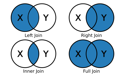
Join

Rather than saying “merge,” dplyr uses the SQL language of joins:

left_join(x, y): keep all x, drop unmatched y
right_join(x, y): keep all y, drop unmatched x
inner_join(x, y): keep only matching
full_join(x, y): keep everything

Joins

Since we want to join a smaller aggregated data frame to the original data frame, we’ll use a left_join(). The join functions will try to guess the joining variable (and tell you what it picked) if you don’t supply one, but we’ll specify one to be clear.

## join on school ID variable
df <- df %>% left_join(sch_m, by = 'sch_id')

Quick exercise

Join the average reading test score data frame you made to the main data object.

Write

The readr library can also write delimited flat files. Instead of write_delim(), we’ll use the wrapper function write_csv() to save a csv file. Again, it’s a good habit to save any modified data using a different name so that your raw data stays untouched. We’ll add _mod_tv to the data name so that we don’t overwrite raw data or the modified data set we made in the last module.

## write flat file
write_csv(df, '../data/els_plans_mod_tv.csv')

Workshop on R

May 2018

Overview
Schedule
Getting started
Modules
Data

Wrangling data II

Tidyverse

Magrittr and pipes

Data wrangling with tidyverse

Mutate

Quick exercise

Select

Quick exercise

Filter

Quick exercise

Arrange

Quick exercise

Summarize

Quick exercise

Join

Quick exercise

Write