Workshop on R
May 2018
Hosted by Virginia Education Science Training (VEST) Program at UVA

Overview Schedule Getting started Modules Data
Web scraping in R
This module introduces the basic steps to scrape data from a website using the rvest. Because there are about as many ways to scrape a website as there are types of web data that you want to gather, web scraping is both art and science, with varying degrees of data cleaning required. If you are lucky, data will be regularly and unambiguously formatted, meaning that it is easy to grab the data you want in the format that you want. If you are less lucky, regular expressions to clean strings will quickly become your friend.
Knowing a bit about web design, specifically HTML, XML, and CSS is helpful when web scraping. This module focuses on static sites, but sites that require user interaction (e.g., clicking a button or inputting data into a form in order to show data) can also be scraped. These sites require special packages such as RSelenium and some knowledge of Javascript is helpful.
For this module, however, we’ll read static web tables from NCES Digest of Education Statistics. NCES helpfully makes these tables available in downloadable Excel worksheets, but we’ll pretend they don’t exist for the moment. Specifically, we’ll focus on Table 302.10, which shows numbers of high school graduates and percentage of college enrollment, broken out by gender and college level, for the years 1960 through 2016.
## libraries
library(tidyverse)
library(rvest)
library(lubridate)
Inspect the web site
First, let’s check out the table we want to scrape. The table we see looks like a regularly formatted table, much like we would see in a paper document. But unlike a printed document, a web page relies on hidden-from-the-user code to generate what we see. By doing it this way instead of serving a static image, websites can adjust to the wide array of user screen sizes, devices, and operating systems. Instructions that tell the user device how to generate the page are also smaller than sending a preformatted image, so bandwidth and time to load are also reduced.
But as web scrapers, we don’t need this. We need the underlying HTML/CSS/XML code used to generate the page. To see it, you’ll need to use a web site inspector. With Firefox and Chrome, you should be able to right-click the page and see the underlying code (you may need to turn on developer tools first). With Safari, you will have to enable the developer tools first.
The top code of the page should look something like this:
<!DOCTYPE html PUBLIC "-//W3C//DTD XHTML 1.0 Transitional//EN" "http://www.w3.org/TR/xhtml1/DTD/xhtml1-transitional.dtd">
<!-- Current year pub navigation function -->
Moving further down, we find the table data, but in a very different format (first row):
...
<tr>
<th class="TblCls009" scope="row" nowrap="nowrap">1960 </th>
<td class="TblCls010">1,679</td>
<td class="TblCls011">(44.5)</td>
<td class="TblCls010">756</td>
<td class="TblCls011">(32.3)</td>
<td class="TblCls010">923</td>
<td class="TblCls011">(30.1)</td>
<td class="TblCls010">45.1</td>
<td class="TblCls011">(2.16)</td>
<td class="TblCls010">—</td>
<td class="TblCls011">(†)</td>
<td class="TblCls010">—</td>
<td class="TblCls011">(†)</td>
<td class="TblCls010">54.0</td>
<td class="TblCls011">(3.23)</td>
<td class="TblCls010">—</td>
<td class="TblCls011">(†)</td>
<td class="TblCls010">—</td>
<td class="TblCls011">(†)</td>
<td class="TblCls010">37.9</td>
<td class="TblCls011">(2.85)</td>
<td class="TblCls010">—</td>
<td class="TblCls011">(†)</td>
<td class="TblCls010">—</td>
<td class="TblCls011">(†)</td>
</tr>
...
The task is to convert these data into a data frame that we can then store or use in tables and figures. This is what the rvest helps us do.
Read web site
The first step is to read the web page code into an object using the
read_html() function.
## set site
url <- 'https://nces.ed.gov/programs/digest/d17/tables/dt17_302.10.asp'

## get site
site <- read_html(url)
Showing our object, we can see that the basic structure of the web page is stored.
## show
site
{xml_document}
<html>
[1] <head>\n<meta http-equiv="Content-Type" content="text/html; charset= ...
[2] <body bgcolor="#ffffff" text="#000000">\r\n\t\r\n\t<!-- Main NCES He ...
Select nodes
Right now, we have a structured, but not particularly useful object
holding our web page data. To pull out specific data, we use the
html_nodes() function. Selecting a node is somewhat akin to using
dplyr::filter() on a data frame.
Great…but what’s a node and how do I know which ones to use? First, a
node is a particular element that is comprised of some information
stored between, for example, HTML tags like <p>...</p> or
<h1>...</h2>. Good web design says that information on page should be
organized by its purpose and similarity to other data. For example,
major headers should be wrapped in <h1> tags and similar page sections
should be given the same CSS class. We can use CSS ids and classes with
the html_nodes() function to pull the exact data we need.
Great!…but what are the classes that we need? Well, we could just inspect the web page manually and guess. For some pages, that works great. But it certainly looks like a chore for this page. Luckily, there’s a great tool that will help us.
SelectorGadget
SelectorGadget is a plugin for the Chrome browser that allows you to click on a web page and, through process of elimination, get the exact combination of HTML tags and CSS ids and classes you need to pull only the data you need.
The SelectorGadget page has instructions, but briefly, this is the process:
- On the first click, SelectorGadget will make its best guess about what you want based on the item you clicked (e.g., table column). The particular element you clicked will be green. The other elements it assumed you want will turn yellow. Sometimes it’s right and you’re finished!
- Often, it will select something you don’t want. In that case, click on the yellow item you don’t want. Again, SelectorGadget will make and informed guess. Sometimes it will drop all extraneous elements and sometimes you will need to click multiple times. These elements will be red.
- On the other hand, SelectorGadget may not have given you everything you want. Keep clicking on new elements (and dropping the extra) until only what you want is highlighted in either green or yellow.
As you’re clicking, you’ll see a box with a string of element ids and
classes changing. When you’re finished, copy this string. This is your
node you’ll use in the html_nodes() function!
Quick exercise
Get the SelectorGadget plugin and play with it for a few minutes. See if you select only a specific column then only a specific row.
First column of data
As a first step, let’s get the first column of data in Table 302.10: the
total number of recent high school graduates. Using SelectorGadget, I
see that the node string I should use is '.tableBracketRow
td:nth-child(2)'. After selecting the node, we use html_text() to
convert the data into a vector like we’re used to seeing.
## subset to just first column
tot <- site %>%
    html_nodes('.tableBracketRow td:nth-child(2)') %>%
    html_text()

## show
tot
 [1] "1,679" "1,763" "1,838" "1,741" "2,145" " "     "2,659" "2,612"
 [9] "2,525" "2,606" "2,842" " "     "2,758" "2,875" "2,964" "3,058"
[17] "3,101" " "     "3,185" "2,986" "3,141" "3,163" "3,160" " "
[25] "3,088" "3,056" "3,100" "2,963" "3,012" " "     "2,668" "2,786"
[33] "2,647" "2,673" "2,450" " "     "2,362" "2,276" "2,397" "2,342"
[41] "2,517" " "     "2,599" "2,660" "2,769" "2,810" "2,897" " "
[49] "2,756" "2,549" "2,796" "2,677" "2,752" " "     "2,675" "2,692"
[57] "2,955" "3,151" "2,937" " "     "3,160" "3,079" "3,203" "2,977"
[65] "2,868" " "     "2,965" "3,137"
So far so good, but we can see a few problems. First, the blank rows in
the table show up in our data. While those blank table spaces are good
for the eyes, they aren’t good in our data set. Let’s try to remove them
using the trim = TRUE option.
## ...this time trim blank spaces
tot <- site %>%
    html_nodes('.tableBracketRow td:nth-child(2)') %>%
    html_text(trim = TRUE)

## show
tot
 [1] "1,679" "1,763" "1,838" "1,741" "2,145" ""      "2,659" "2,612"
 [9] "2,525" "2,606" "2,842" ""      "2,758" "2,875" "2,964" "3,058"
[17] "3,101" ""      "3,185" "2,986" "3,141" "3,163" "3,160" ""
[25] "3,088" "3,056" "3,100" "2,963" "3,012" ""      "2,668" "2,786"
[33] "2,647" "2,673" "2,450" ""      "2,362" "2,276" "2,397" "2,342"
[41] "2,517" ""      "2,599" "2,660" "2,769" "2,810" "2,897" ""
[49] "2,756" "2,549" "2,796" "2,677" "2,752" ""      "2,675" "2,692"
[57] "2,955" "3,151" "2,937" ""      "3,160" "3,079" "3,203" "2,977"
[65] "2,868" ""      "2,965" "3,137"
Better, but the empty elements are still there. Luckily, we can just use base R to remove them.
## remove blank values
tot <- tot[tot != '']

## show
tot
 [1] "1,679" "1,763" "1,838" "1,741" "2,145" "2,659" "2,612" "2,525"
 [9] "2,606" "2,842" "2,758" "2,875" "2,964" "3,058" "3,101" "3,185"
[17] "2,986" "3,141" "3,163" "3,160" "3,088" "3,056" "3,100" "2,963"
[25] "3,012" "2,668" "2,786" "2,647" "2,673" "2,450" "2,362" "2,276"
[33] "2,397" "2,342" "2,517" "2,599" "2,660" "2,769" "2,810" "2,897"
[41] "2,756" "2,549" "2,796" "2,677" "2,752" "2,675" "2,692" "2,955"
[49] "3,151" "2,937" "3,160" "3,079" "3,203" "2,977" "2,868" "2,965"
[57] "3,137"
Getting closer. Next, let’s convert our numbers to actual numbers, which
R thinks are strings at the moment. To do this, we need to get rid of
the commas. The gsub() function is perfect for this. It’s commands
take the form: gsub('<regular expression to remove>', '<regular
expression to substitute in place of old>', <variable>). Regular
expressions can become complicated, but our use here is simple:
## remove commas, replacing with empty string
tot <- gsub(',', '', tot)

## show
tot
 [1] "1679" "1763" "1838" "1741" "2145" "2659" "2612" "2525" "2606" "2842"
[11] "2758" "2875" "2964" "3058" "3101" "3185" "2986" "3141" "3163" "3160"
[21] "3088" "3056" "3100" "2963" "3012" "2668" "2786" "2647" "2673" "2450"
[31] "2362" "2276" "2397" "2342" "2517" "2599" "2660" "2769" "2810" "2897"
[41] "2756" "2549" "2796" "2677" "2752" "2675" "2692" "2955" "3151" "2937"
[51] "3160" "3079" "3203" "2977" "2868" "2965" "3137"
Now we’re ready to convert to a number.
## convert to numeric
tot <- as.integer(tot)

## show
tot
 [1] 1679 1763 1838 1741 2145 2659 2612 2525 2606 2842 2758 2875 2964 3058
[15] 3101 3185 2986 3141 3163 3160 3088 3056 3100 2963 3012 2668 2786 2647
[29] 2673 2450 2362 2276 2397 2342 2517 2599 2660 2769 2810 2897 2756 2549
[43] 2796 2677 2752 2675 2692 2955 3151 2937 3160 3079 3203 2977 2868 2965
[57] 3137
Finished!
Add year
So that these numbers make sense, let’s grab the years column and create
and data frame so that we can make a figure of long term high school
completer totals. Again, the first step is to use SelectorGadget to get
the node string. This time, it’s 'tbody th'.
## get years column
years <- site %>%
    html_nodes('tbody th') %>%
    html_text(trim = TRUE)

## remove blank spaces like before
years <- years[years != '']

## show
years
 [1] "1960"  "1961"  "1962"  "1963"  "1964"  "1965"  "1966"  "1967"
 [9] "1968"  "1969"  "1970"  "1971"  "1972"  "1973"  "1974"  "1975"
[17] "1976"  "1977"  "1978"  "1979"  "1980"  "1981"  "1982"  "1983"
[25] "1984"  "1985"  "1986"  "1987"  "1988"  "1989"  "1990"  "1991"
[33] "1992"  "1993"  "1994"  "1995"  "1996"  "1997"  "1998"  "1999"
[41] "2000"  "2001"  "2002"  "2003"  "2004"  "2005"  "2006"  "2007"
[49] "2008"  "2009"  "20103" "20113" "20123" "20133" "20143" "20153"
[57] "20163"
We’ve gotten rid of the blank items, but now we have a new problem: the
footnotes in the last few years has just be added to the year. Instead
of 2010, we have 20103, and so on through 2016. Since the problem is
small (it’s easy to see all the bad items) and regular (always extra 3
as the 5th digit), we can fix it using substring().
## trim footnote that's become extra digit
years <- substring(years, 1, 4)

## show
years
 [1] "1960" "1961" "1962" "1963" "1964" "1965" "1966" "1967" "1968" "1969"
[11] "1970" "1971" "1972" "1973" "1974" "1975" "1976" "1977" "1978" "1979"
[21] "1980" "1981" "1982" "1983" "1984" "1985" "1986" "1987" "1988" "1989"
[31] "1990" "1991" "1992" "1993" "1994" "1995" "1996" "1997" "1998" "1999"
[41] "2000" "2001" "2002" "2003" "2004" "2005" "2006" "2007" "2008" "2009"
[51] "2010" "2011" "2012" "2013" "2014" "2015" "2016"
Fixed! Now we bind together with our high school completers total. Because we want to make a time period line graph, we’ll also convert the years to a data format.
NB Since we dropped blank elements in each vector separately, it’s important to check that all the data line up properly now that we’ve bound them together. If we wanted to be safer, we could have bound the data first, then dropped the rows with double missing values.
## put in data frame
df <- bind_cols(years = years, total = tot) %>%
    mutate(years = as.Date(years, format = '%Y'))
df
# A tibble: 57 x 2
   years      total
   <date>     <int>
 1 1960-12-27  1679
 2 1961-12-27  1763
 3 1962-12-27  1838
 4 1963-12-27  1741
 5 1964-12-27  2145
 6 1965-12-27  2659
 7 1966-12-27  2612
 8 1967-12-27  2525
 9 1968-12-27  2606
10 1969-12-27  2842
# ... with 47 more rows
You can see that the date format adds a month and day (the day the script was run if not supplied). While these particular dates probably aren’t right, we won’t use them later when graphing so they can stay.
Let’s plot our trends.
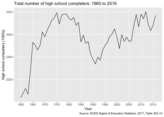
## plot
g <- ggplot(df, mapping = aes(x = years, y = total)) +
    geom_line() +
    scale_x_date(breaks = seq(min(df$years), max(df$years), '5 years'),
                 minor_breaks = seq(min(df$years), max(df$years), '1 years'),
                 date_labels = '%Y') +
    labs(x = 'Year',
         y = 'High school completers (1000s)',
         title = 'Total number of high school completers: 1960 to 2016',
         caption = 'Source: NCES Digest of Education Statistics, 2017, Table 302.10')
g
Quick exercise
Pull in total percentage of enrollment (column 5), add to data frame, and plot against year.
Scrape entire table
Now that we’ve pulled two columns, let’s try to grab the entire table. Once again, we’ll use SelectorGadget to get our node string.
## save node
node <- paste0('.TblCls002 , td.TblCls005 , tbody .TblCls008 , ',
               '.TblCls009 , .TblCls011 , .TblCls010')

## save more dataframe-friendly column names
nms <- c('year','hs_comp_tot', 'hs_comp_tot_se',
         'hs_comp_m', 'hs_comp_m_se',
         'hs_comp_f', 'hs_comp_f_se',
         'enr_pct', 'enr_pct_se',
         'enr_pct_2', 'enr_pct_2_se',
         'enr_pct_4', 'enr_pct_4_se',
         'enr_pct_m', 'enr_pct_m_se',
         'enr_pct_2_m', 'enr_pct_2_m_se',
         'enr_pct_4_m', 'enr_pct_4_m_se',
         'enr_pct_f', 'enr_pct_f_se',
         'enr_pct_2_f', 'enr_pct_2_f_se',
         'enr_pct_4_f', 'enr_pct_4_f_se')

## whole table
tab <- site %>%
    ## use nodes
    html_nodes(node) %>%
    ## to text with trim
    html_text(trim = TRUE)

## show first few elements
tab[1:30]
 [1] "1960"   "1,679"  "(44.5)" "756"    "(32.3)" "923"    "(30.1)"
 [8] "45.1"   "(2.16)" "—"      "(†)"    "—"      "(†)"    "54.0"
[15] "(3.23)" "—"      "(†)"    "—"      "(†)"    "37.9"   "(2.85)"
[22] "—"      "(†)"    "—"      "(†)"    "1961"   "1,763"  "(46.7)"
[29] "790"    "(33.7)"
Okay. It looks like we have it, but it’s all in single dimension vector. Since we eventually want a data frame, let’s convert to a matrix.
## convert to matrix
tab <- tab %>%
    matrix(., ncol = 25, byrow = TRUE)

## dimensions
dim(tab)
[1] 68 25
## show first few columns
tab[1:10,1:10]
      [,1]   [,2]    [,3]     [,4]    [,5]     [,6]    [,7]     [,8]
 [1,] "1960" "1,679" "(44.5)" "756"   "(32.3)" "923"   "(30.1)" "45.1"
 [2,] "1961" "1,763" "(46.7)" "790"   "(33.7)" "973"   "(31.8)" "48.0"
 [3,] "1962" "1,838" "(44.3)" "872"   "(32.0)" "966"   "(30.4)" "49.0"
 [4,] "1963" "1,741" "(44.9)" "794"   "(32.6)" "947"   "(30.5)" "45.0"
 [5,] "1964" "2,145" "(43.6)" "997"   "(32.3)" "1,148" "(28.9)" "48.3"
 [6,] ""     ""      ""       ""      ""       ""      ""       ""
 [7,] "1965" "2,659" "(48.5)" "1,254" "(35.7)" "1,405" "(32.5)" "50.9"
 [8,] "1966" "2,612" "(45.7)" "1,207" "(34.4)" "1,405" "(29.5)" "50.1"
 [9,] "1967" "2,525" "(38.5)" "1,142" "(28.9)" "1,383" "(24.7)" "51.9"
[10,] "1968" "2,606" "(38.0)" "1,184" "(28.7)" "1,422" "(24.2)" "55.4"
      [,9]     [,10]
 [1,] "(2.16)" "—"
 [2,] "(2.12)" "—"
 [3,] "(2.08)" "—"
 [4,] "(2.12)" "—"
 [5,] "(1.92)" "—"
 [6,] ""       ""
 [7,] "(1.73)" "—"
 [8,] "(1.74)" "—"
 [9,] "(1.44)" "—"
[10,] "(1.41)" "—"
Quick exercise
What happens if you don’t use
byrow = TRUEin the matrix command?
It’s getting better, but now we have a lot of special characters that we need to clean out. This section relies more heavily on regular expressions, but the idea is the same as above.
## clean up table
tab <- tab %>%
    ## remove commas
    gsub(',', '', .) %>%
    ## remove dagger and parentheses
    gsub('\\(\U2020\\)', NA, .) %>%
    ## remove hyphens
    gsub('\U2014', NA, .) %>%
    ## remove parentheses, but keep any content that was inside
    gsub('\\((.*)\\)', '\\1', .) %>%
    ## remove blank strings (^ = start, $ = end, so ^$ = start to end w/ nothing)
    gsub('^$', NA, .) %>%
    ## convert to table
    tbl_df() %>%
    ## rename using names above
    setNames(nms) %>%
    ## drop rows with missing year (blank online)
    drop_na(year) %>%
    ## fix years like above
    mutate(year = substring(year, 1, 4)) %>%
    ## convert to numbers
    mutate_all(.funs = funs(as.numeric(.)))

## show
tab
# A tibble: 57 x 25
    year hs_comp_tot hs_comp_tot_se hs_comp_m hs_comp_m_se hs_comp_f
   <dbl>       <dbl>          <dbl>     <dbl>        <dbl>     <dbl>
 1  1960        1679           44.5       756         32.3       923
 2  1961        1763           46.7       790         33.7       973
 3  1962        1838           44.3       872         32         966
 4  1963        1741           44.9       794         32.6       947
 5  1964        2145           43.6       997         32.3      1148
 6  1965        2659           48.5      1254         35.7      1405
 7  1966        2612           45.7      1207         34.4      1405
 8  1967        2525           38.5      1142         28.9      1383
 9  1968        2606           38        1184         28.7      1422
10  1969        2842           36.6      1352         27.3      1490
# ... with 47 more rows, and 19 more variables: hs_comp_f_se <dbl>,
#   enr_pct <dbl>, enr_pct_se <dbl>, enr_pct_2 <dbl>, enr_pct_2_se <dbl>,
#   enr_pct_4 <dbl>, enr_pct_4_se <dbl>, enr_pct_m <dbl>,
#   enr_pct_m_se <dbl>, enr_pct_2_m <dbl>, enr_pct_2_m_se <dbl>,
#   enr_pct_4_m <dbl>, enr_pct_4_m_se <dbl>, enr_pct_f <dbl>,
#   enr_pct_f_se <dbl>, enr_pct_2_f <dbl>, enr_pct_2_f_se <dbl>,
#   enr_pct_4_f <dbl>, enr_pct_4_f_se <dbl>
Got it!
Reshape data
We could stop where we are, but to make the data more usable in the future, let’s convert to a long data frame. This takes a couple of steps, but the idea is to have each row represent a year by estimate, with a column for the estimate value and a column for the standard error on that estimate. It may help to run the code below one line at a time, checking the progress at each step.
## gather for long data
df <- tab %>%
    ## gather estimates, leaving standard errors wide for the moment
    gather(group, estimate, -c(year, ends_with('se'))) %>%
    ## gather standard errors
    gather(group_se, se, -c(year, group, estimate)) %>%
    ## drop '_se' from standard error estimates
    mutate(group_se = gsub('_se', '', group_se)) %>%
    ## filter where group == group_se
    filter(group == group_se) %>%
    ## drop extra column
    select(-group_se) %>%
    ## arrange
    arrange(year)

df
# A tibble: 684 x 4
    year group       estimate    se
   <dbl> <chr>          <dbl> <dbl>
 1  1960 hs_comp_tot   1679   44.5
 2  1960 hs_comp_m      756   32.3
 3  1960 hs_comp_f      923   30.1
 4  1960 enr_pct         45.1  2.16
 5  1960 enr_pct_2       NA   NA
 6  1960 enr_pct_4       NA   NA
 7  1960 enr_pct_m       54    3.23
 8  1960 enr_pct_2_m     NA   NA
 9  1960 enr_pct_4_m     NA   NA
10  1960 enr_pct_f       37.9  2.85
# ... with 674 more rows
Plot trends
Let’s look at overall college enrollment percentages for recent graduates over time. Because our data are nicely formatted, it’s easy to subset the full table to data to only those estimates we need as well as generate 95% confidence intervals.
## adjust data for specific plot
plot_df <- df %>%
    filter(group %in% c('enr_pct', 'enr_pct_m', 'enr_pct_f')) %>%
    mutate(hi = estimate + se * qnorm(.975),
           lo = estimate - se * qnorm(.975),
           year = as.Date(as.character(year), format = '%Y'),
           group = ifelse(group == 'enr_pct_f', 'Women',
                   ifelse(group == 'enr_pct_m', 'Men', 'All')))

## show
plot_df
# A tibble: 171 x 6
   year       group estimate    se    hi    lo
   <date>     <chr>    <dbl> <dbl> <dbl> <dbl>
 1 1960-12-27 All       45.1  2.16  49.3  40.9
 2 1960-12-27 Men       54    3.23  60.3  47.7
 3 1960-12-27 Women     37.9  2.85  43.5  32.3
 4 1961-12-27 All       48    2.12  52.2  43.8
 5 1961-12-27 Men       56.3  3.14  62.5  50.1
 6 1961-12-27 Women     41.3  2.81  46.8  35.8
 7 1962-12-27 All       49    2.08  53.1  44.9
 8 1962-12-27 Men       55    3     60.9  49.1
 9 1962-12-27 Women     43.5  2.84  49.1  37.9
10 1963-12-27 All       45    2.12  49.2  40.8
# ... with 161 more rows
First, let’s plot the overall average. Notice that we use the filter()
function in the ggplot() function to remove the subgroup estimates for
men and women.
## plot overall average
g <- ggplot(plot_df %>% filter(group == 'All'),
            mapping = aes(x = year, y = estimate)) +
    geom_ribbon(aes(ymin = lo, ymax = hi), fill = 'grey70') +
    geom_line() +
    scale_x_date(breaks = seq(min(plot_df$year), max(plot_df$year),
                              '5 years'),
                 minor_breaks = seq(min(plot_df$year), max(plot_df$year),
                                    '1 years'),
                 date_labels = '%Y') +
    labs(x = 'Year',
         y = 'Percent',
         title = 'Percent of recent high school completers in college: 1960 to 2016',
         caption = 'Source: NCES Digest of Education Statistics, 2017, Table 302.10')
g
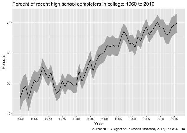
After a small dip in the early 1970s (once the Baby Boom generation had largely left college), enrollment trends have steadily risen over time.
Now let’s compare enrollments over time between men and women (dropping the overall average so our plot is clearer).
## plot comparison between men and women
g <- ggplot(plot_df %>% filter(group %in% c('Men','Women')),
            mapping = aes(x = year, y = estimate, colour = group)) +
    geom_ribbon(aes(ymin = lo, ymax = hi, fill = group), alpha = 0.2) +
    geom_line() +
    scale_x_date(breaks = seq(min(plot_df$year),
                              max(plot_df$year),
                              '5 years'),
                 minor_breaks = seq(min(plot_df$year),
                                    max(plot_df$year),
                                    '1 years'),
                 date_labels = '%Y') +
    labs(x = 'Year',
         y = 'Percent',
         title = 'Percent of recent high school completers in college: 1960 to 2016',
         caption = 'Source: NCES Digest of Education Statistics, 2017, Table 302.10') +
    guides(fill = guide_legend(title = 'Group'),
           colour = FALSE) +
    theme(legend.position = c(1,0), legend.justification = c(1,0))
g
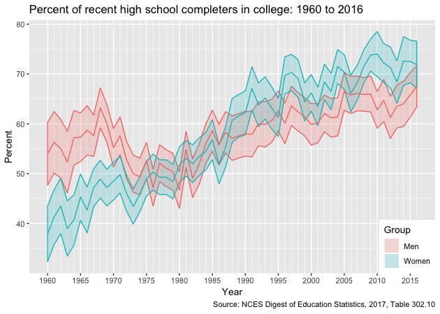
Though a greater proportion of men enrolled in college in the 1960s and early 1970s, women have been increasing their enrollment percentages faster than men since the 1980s and now have comparatively higher rates of college participation.
Not-so-quick exercise
Find the unemployment rate for 25 to 34 year-olds by degree type for the years 2010 through 2016. Make a long data frame that can be saved or used to make a figure of trends over time by educational attainment.
See Table 501.10 of the NCES Digest of Education Statistics, which can can be found here. (HINT: notice the structure of the url for the 2017 year table and the 2016; once you’ve got one to work, can you write a loop?)