Workshop on R
May 2018
Hosted by Virginia Education Science Training (VEST) Program at UVA

Overview Schedule Getting started Modules Data
Programming in R II
In this module, we’ll continue to practice functional programming in R.
To give us something to work on, we’ll code up our own version of a
k-means clustering
algorithm. R already has a function to do this, appropriately titled
kmeans(), but we’ll pretend it doesn’t.
Being able to code up an algorithm based on mathematical notation or pseudocode is a really valuable skill to possess. As algorithms become even moderately complex, however, leaning on quick and dirty spaghetti code to “just get the job done” quickly becomes a mess. When you’ve worked hard to get an algorithm to work, it’s important to work a little harder to write it in a functional way that
- Makes it clear what you have done (self-documenting);
- Is easily ported to another project.
With these goals in mind, we’ll write our own k-means clustering function. Because this lesson isn’t about learning the ins and outs of machine learning, we won’t dive into the various robustness checks we might otherwise perform were this a real project. That said, we should be able to write a well-performing function.
## libraries
library(tidyverse)
library(plotly)
Read in and inspect data
As always, our first step after loading our libraries is to load our data.
## read in data
df <- readRDS('../data/programming_two.rds')

## show
df
# A tibble: 1,500 x 3
        x     y     z
    <dbl> <dbl> <dbl>
 1  33.1  11.6  -16.0
 2  -8.55  6.01  11.8
 3  50.7  56.3   97.8
 4   2.83 27.5   34.4
 5  -4.66 20.0   25.1
 6  -3.04 16.2   22.8
 7  30.5  12.1  -14.3
 8   7.08 25.3   25.6
 9   1.33 20.1   17.6
10  -3.11 13.4   11.5
# ... with 1,490 more rows
The data set is an 1,500 by 3 matrix, with three covariates (or features
in machine learning parlance), x, y, and z. Since these columns
names don’t tell us much, let’s plot the first two features against each
other in a scatter plot.
## plot first two dimensions
g <- ggplot(df, mapping = aes(x = x, y = y)) + geom_point()
g
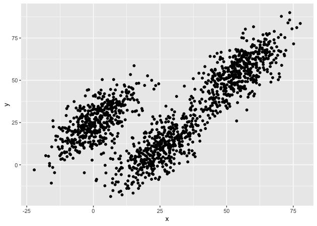
While there appears to be an overall positive correlation between x
and y, the data seem to cluster into three groups. One group (furthest
left on the x axis) seems more distinct from the other two, which look
to be on the same trend line, but clumped in lower and higher positions.
Our task will be to assign each point to an as yet unspecified group with the goal that each group will be contiguous (e.g., will cluster together).
K-means clustering
Formally, the objective function for a k-means clustering algorithm is as follows (from Wikipedia):
\[ \underset{S}{arg\,min} \sum_{i=1}^k\sum_{x\in S_i} \vert\vert x - \mu_i \vert\vert^2\]
where
- \(k\) is the number of clusters
- \(S_i\) is one cluster set of points
- \(\vert\vert x - \mu_i \vert\vert^2\) is the squared Euclidean distance
In English, the objective is that for a fixed number of clusters, assign each point to a cluster such the variance within each cluster (within-cluster sum of squares or WCSS) is minimized. If you think that this sounds like the objective of ordinary least squares (OLS), you are right. The difference here is that instead of creating a line of best fit (or using parametric assumptions to make inferences), we are simply assigning each point to its “cluster of best fit.”
Algorithm
There are number of algorithms to compute k-means. We’ll use Lloyd’s algorithm, which isn’t the best, but is the simplest and works well enough for our purposes.
- Choose number of clusters, \(k\).
- Randomly choose \(k\) points from data to serve as initial cluster means.
- Repeat following steps until assignments no longer change:
- Assign each point to the cluster with the closest mean (see Step 3.1, below, for formal definition).
- Update means to reflect points assigned to the cluster (see Step 3.2, below, for formal definition).
Step 3.1: Assign each point to the closest mean
\[ S_i^{(t)} = \{ x_p : \vert\vert x_p - m_i^{(t)} \vert\vert^2 \leq \vert\vert x_p - m_j^{(t)} \vert\vert^2 \,\forall\, j, 1 \lt j \lt k \}\]
At time \(t\), each set, \(S_i\), contains all the points, \(x_p\) for which its mean, \(m_i^{(t)}\), is the nearest of possible cluster means.
Step 3.2: Update means to reflect points in the cluster
\[ m_i^{(t+1)} = \frac{1}{\vert S_i^{(t)} \vert} \sum_{x_j\in S_i^{(t)}} x_j \]
At time \(t+1\), each cluster mean \(m_i^{(t+1)}\) is the centroid of the points, \(x_j\) assigned to the cluster at time \(t\).
Let’s just get it to run!
For our first step, let’s see if we can “just get the job done.” With
that in mind, we’ll limit the number of features to two, x and
y.
## convert data to matrix to make our lives easier (x and y, only, for now)
dat <- df %>% select(x, y) %>% as.matrix()
As the first step, we need to pick some means. We’ll do this by sampling 3 numbers between 1 and the number of rows in the data frame (1,500). Next we’ll use these to pull out three rows that will be our starting means.
## get initial means to start
index <- sample(1:nrow(dat), 3)           # give k random indexes
means <- dat[index,]

## show
means
             x         y
[1,] 54.880387  53.09005
[2,]  8.153264 -11.72703
[3,] -1.864422  13.26329
Next, we need to keep track of how we assign each point. To that end, we
will first initialize an empty numeric vector with a spot for each
point, assign_vec. After that, we’ll loop through each point, compute
the distance between that point and each mean, and put the index of the
closest mean (effectively the label) in the point’s spot in
assign_vec. For example, if the first point is closest to the first
mean, assign_vec[1] == 1; if the 10th point is closest to the third
mean, assign_vec[10] == 3, and so on.
## init assignment vector
assign_vec <- numeric(nrow(dat))

## assign each point to one of the clusters
for (i in 1:nrow(dat)) {
    ## init a temporary distance object to hold k distance values
    distance <- numeric(3)
    ## compare to each mean
    for (j in 1:3) {
        distance[j] <- sum((dat[i,] - means[j,])^2)
    }
    ## assign the index of smallest value,
    ## which is effectively cluster ID
    assign_vec[i] <- which.min(distance)
}

## show first few
assign_vec[1:20]
[1] 2 3 1 3 3 3 3 3 3 3 3 1 1 1 3 1 3 2 3 1
Quick exercise
Merge the assignments back to the data (everything should be in order for a quick
cbind()orbind_cols()) and then plot, assigning a unique color to each group. How did we do the first iteration?
Okay, we’ve started, but our means were arbitrary and probably weren’t the best. Now we need to pick new means and repeat the code above. We need to keep doing this until the assignments don’t change.
A while() loop is perfect for this task. We’ll create a variable
called identical, which will take the Boolean FALSE. While
identical is not FALSE (i.e., TRUE), the loop will continue.
Inside, we’ll compute new means, store the assignments in another object
so that we can compare later, run the same code as above again, then
compare the old and the new. If the old and new assignments are
different, then identical remains FALSE and the loop runs again. If
the old and new assignments are the same, however, identical becomes
TRUE and the loop stops because !TRUE == FALSE.
## repeat above in loop until assignments don't change
identical <- FALSE
while (!identical) {

    ## update means by subsetting each column
    ## by assignment group, taking mean
    for (i in 1:3) {
        means[i,] <- colMeans(dat[assign_vec == i,])
    }

    ## store old assignments, b/c we need to compare
    old_assign_vec <- assign_vec

    ## assign each point to one of the clusters
    for (i in 1:nrow(dat)) {
        ## init a temporary distance object
        ## to hold k distance values
        distance <- numeric(3)
        ## compare to each mean
        for (j in 1:3) {
            distance[j] <- sum((dat[i,] - means[j,])^2)
        }
        ## assign the index of smallest value,
        ## which is effectively cluster ID
        assign_vec[i] <- which.min(distance)
    }

    ## check if assignments change
    identical <- identical(old_assign_vec, assign_vec)
}
Let’s check to see how we did.
## check assignment with scatter plot
plot_df <- bind_cols(df, as.data.frame(assign_vec))
g <- ggplot(plot_df, mapping = aes(x = x, y = y,
                                   color = factor(assign_vec))) +
    geom_point()
g
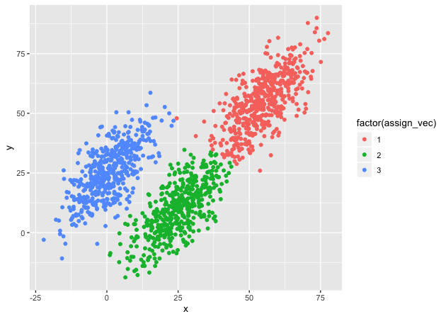
Looks like we did it! The clusters are, well, clustered and the points, for the most part, seem to be labeled correctly.
Quick exercise
The k-means algorithm can be sensitive to the starting points since it finds locally optimal solutions (no guarantee that the solution is the best of all possible solutions). Run the code again a couple of times and see how your fit changes. Do some points move between groups?
Problems
Our success not withstanding, we have a number of problems:
- We have exactly repeated code
- Magic numbers in the code (3)
- Variable names that depend on working environment
- Primary purpose of code is obfuscated
Problems 1-3 make it difficult to change things in the code. We have to remember and find each repeated instance that we want to change. Problem 3 makes it difficult to re-use the code in another script (who knows what global variables are currently lurking and, once gone, will mess up our program?).
Problem 4 means that it will be difficult to see what we did when coming back to the code in the future. With the repeated steps and the loop, it will be easy to lose the forest for the trees. What’s the point of this section of code again? After reading through multiple lines, we’ll see, if we’re lucky, that we were running a k-means clustering algorithm. That’s wasted time.
Convert to functions
What we need is to convert our spaghetti code to DRY (don’t repeat yourself) code. Each unique bit of code should be wrapped in function that does one thing and does it well. Since functions can use other functions, we can start at the smallest part and build up to something more complex.
What do we need? Looking at the code above, it looks like we would benefit from having unique functions to:
- compute squared Euclidean distance
- compute new means based on assignment labels
- make new cluster assignments for each point
Euclidean distance function
## Euclidean distance^2
euclid_dist_sq <- function(x,y) return(sum((x - y)^2))
Compute means
## compute new means for points in cluster
compute_mean <- function(data, k, assign_vec) {
    ## init means matrix: # means X # features (data columns)
    means <- matrix(NA, k, ncol(data))
    ## for each mean, k...
    for (i in 1:k) {
        ## ...get column means, restricting to cluster assigned points
        means[i,] <- colMeans(data[assign_vec == i,])
    }
    return(means)
}
Make new assignments
Notice that we’ve added a bit to our code above. We might find it useful
to compute the within-cluster sum of squares (WCSS), so we’ve added and
object, wcss, that has one spot for each cluster and holds a running
total of the sum of squares within each cluster.
To return multiple objects from a function, R requires that they be stored in a list. This function will return both the assignments for each point, like before, as well as the WCSS.
## find nearest mean to each point and assign to cluster
assign_to_cluster <- function(data, k, means, assign_vec) {
    ## init within-cluster sum of squares for each cluster
    wcss <- numeric(k)
    ## for each data point (slow!)...
    for (i in 1:nrow(data)) {
        ## ...init distance vector, one for each cluster mean
        distance <- numeric(k)
        ## ...for each mean...
        for (j in 1:k) {
            ## ...compute distance to point
            distance[j] <- euclid_dist_sq(data[i,], means[j,])
        }
        ## ...assign to cluster with nearest mean
        assign_vec[i] <- which.min(distance)
        ## ...add distance to running sum of squares
        ## for assigned cluster
        wcss[assign_vec[i]] <- wcss[assign_vec[i]] + distance[assign_vec[i]]
    }
    return(list('assign_vec' = assign_vec, 'wcss' = wcss))
}
BONUS: standardize data
Many machine learning algorithms perform better if the covariates are on the same scale. We’ve not really had to worry about this so far since our data are scaled roughly the same. That said, we may want to use this algorithm in the future with data that aren’t similarly scaled (say, on data with age in years and family income in dollars).
This function simply standardizes a matrix of data and returns the scaled data along with the mean and standard deviations of each column (feature), which are useful for rescaling the data later.
## standardize function that also returns mu and sd
standardize <- function(data) {
    ## column means
    mu <- colMeans(data)
    ## column standard deviations
    sd <- sqrt(diag(var(data)))
    ## scale data (z-score); faster to use pre-computed mu/sd
    sdata <- scale(data, center = mu, scale = sd)
    return(list('mu' = mu, 'sd' = sd, 'scaled_data' = sdata))
}
K-means function
Now that we have the pieces, we can put the pieces together in single function. Our function takes the following arguments:
data: a data frame (converted to matrix inside the function)k: number of clusters we wantiterations: a stop valve in case our algorithm doesn’t want to convergenstarts: a new feature that says how many times to start the algorithm; while not perfect it may help prevent some sub-optimal local solutionsstandardize: an option to standardize the data
Note that only data and k have to be supplied by the user. The other
arguments have default values. If we leave them out of the function
call, the defaults will be used.
## k-means function
my_kmeans <- function(data,                  # data frame
                      k,                     # number of clusters
                      iterations = 100,      # max iterations
                      nstarts = 1,           # how many times to run
                      standardize = FALSE) { # standardize data?

    ## convert to matrix
    x <- as.matrix(data)

    ## standardize if TRUE
    if (standardize) {
        sdata <- standardize(data)
        x <- sdata[['scaled_data']]
    }

    ## for number of starts
    for (s in 1:nstarts) {

        ## init identical
        identical <- FALSE

        ## select k random points as starting means
        means <- x[sample(1:nrow(x),k),]

        ## init assignment vector
        init_assign_vec <- rep(NA, nrow(x))

        ## first assignment
        assign_wcss <- assign_to_cluster(x, k, means, init_assign_vec)

        ## iterate until iterations run out
        ## or no change in assignment
        while (iterations > 0 && !identical) {

            ## store old assignment / wcss object
            old_assign_wcss <- assign_wcss

            ## get new means
            means <- compute_mean(x, k,
                                  assign_wcss[['assign_vec']])

            ## new assignments
            assign_wcss <- assign_to_cluster(x, k, means,
                                             assign_wcss[['assign_vec']])

            ## check if identical (no change in assignment)
            identical <- identical(old_assign_wcss[['assign_vec']],
                                   assign_wcss[['assign_vec']])

            ## reduce iteration counter
            iterations <- iterations - 1
        }

        ## store best values...
        if (s == 1) {
            best_wcss <- assign_wcss[['wcss']]
            best_centers <- means
            best_assignvec <- assign_wcss[['assign_vec']]
        } else {
            ## ...update accordingly if number of starts is > 1
            ## & wcss is lower
            if (sum(assign_wcss[['wcss']]) < sum(best_wcss)) {
                best_wcss <- assign_wcss[['wcss']]
                best_centers <- means
                best_assignvec <- assign_wcss[['assign_vec']]
            }
        }
    }

    ## convert back to non-standard centers if necessary
    if (standardize) {
        sd <- sdata[['sd']]
        mu <- sdata[['mu']]
        for (j in 1:ncol(x)) {
            best_centers[,j] <- best_centers[,j] * sd[j] + mu[j]
        }
    }

    ## return assignment vector, cluster centers, & wcss
    return(list('assignments' = best_assignvec,
                'centers' = best_centers,
                'wcss' = best_wcss))
}
Quick exercise
Look through the function and talk through how the function will run with the following arguments:
my_kmeans(data, 3)my_kmeans(data, 3, standardize = TRUE)my_kmeans(data, 3, nstarts = 10)
2 dimensions
Now that we have our proper function, let’s run it! Let’s go back to where we started, with two dimensions.
## 2 dimensions
km_2d <- my_kmeans(data = df[,c('x','y')], k = 3, nstarts = 20)

## check assignments, centers, and wcss
km_2d$assignments[1:20]
[1] 1 2 3 2 2 2 1 2 2 2 2 3 3 3 2 1 2 1 1 3
km_2d$centers
           [,1]      [,2]
[1,] 25.0407539  9.780767
[2,]  0.7741392 25.471911
[3,] 54.6683528 54.725368
km_2d$wcss
[1] 88179.39 89184.79 99748.81
Notice how clear and unambiguous our code is now. We are running a k-means clustering algorithm with three clusters. We get results that tell us the assignments for each point, the centers of the clusters, and the WCSS.
3 dimensions
The nice thing about our function is that it easily scales to more than two dimensions. Instead of subsetting the data, we’ll just include it all for 3 dimensions this time.
## 3 dimensions
km_3d <- my_kmeans(data = df, k = 3, nstarts = 20)

## check centers and wcss
km_3d$assignments[1:20]
[1] 1 2 3 2 2 2 1 2 2 2 2 3 3 3 2 1 2 1 1 3
km_3d$centers
           [,1]     [,2]      [,3]
[1,] 25.2858908 10.26503 -24.21246
[2,]  0.8928973 25.51276  25.58783
[3,] 54.8865406 54.97876 105.13575
km_3d$wcss
[1] 167007.1 153343.3 159247.5
Check out plots
Let’s plot our assignments. First, let’s plot the two dimensional assignments. We’ll use plotly this time so that it’s easier to zoom in on individual points.
## using 2D: looks good 2D...
p <- plot_ly(df, x = ~x, y = ~y, color = factor(km_2d$assignments)) %>%
    add_markers()
p
Looks pretty much like our first plot above. But what happens if we
include the third feature, z, that we ignored?
## ...but off in 3D
p <- plot_ly(df, x = ~x, y = ~y, z = ~z, color = factor(km_2d$assignments),
             marker = list(size = 3)) %>%
    add_markers()
p
Ah! Not so good! Clearly, some of the points appear to fit in one
cluster if only x and y are considered, but no longer do when the
third dimension is included.
Quick exercise
Manipulate the 3D plotly figure to see if you can recreate the 2D plot, that is adjust the viewing angle. Then move it around to see how that flattened view was deceptive.
Let’s move to our results that used all three features. Again, we’ll first look in just two dimensions.
## using 3D: looks off in 2D...
p <- plot_ly(df, x = ~x, y = ~y, color = factor(km_3d$assignments)) %>%
    add_markers()
p
In two dimensions, our clusters look a bit messy since they overlap on the edges. But looking in three dimensions…
## ...but clearly better fit in 3D
p <- plot_ly(df, x = ~x, y = ~y, z = ~z, color = factor(km_3d$assignments),
             marker = list(size = 3)) %>%
    add_markers()
p
Much better! Not perfect, but better.