High performance R with Rcpp

R is really powerful, but for some tasks can be very slow. As data get larger and scripts require more complex algorithms and demanding tasks, even small bits of sluggishness become huge in the aggregate. Compiled languages such as C and C++ can be much faster than R, but require greater programming skill. While learning a compiled language is useful for many researchers, the upfront time needed to learn is often too steep for any given project.

Fortunately, the Rcpp package bridges the gap between the two worlds. While there is a bit of a learning curve for Rcpp, which is based on C++, much R code can be, with few modifications, adjusted to become Rcpp code and run much faster for complex tasks.

This module will give one example of such a speed up. In my own research, I’ve computed the Great Circle (“as the crow flies”) distance between colleges and various geographic centroids many times using either the Haversine or Vincenty formula. But with over 7,500 colleges and universities in the United States, measuring the distance from each county centroid (around 3,000) became slow enough. Doing the same for all census tracks (around 70,000) and census block groups (over 200,000) was almost impossible. With small modifications to base R formula functions, however, I was able to convert them to compiled Rcpp function which run much, much faster.

## libraries
library(tidyverse)
library(Rcpp)
library(microbenchmark)

Load data

This module uses two data frames. The first has the names and locations of all colleges with a physical campus in 2015. The second has the locations of every census block group in the United States from the 2010 Census.

## load data
load('../data/hp_rcpp.Rdata')

College locations

Here’s a quick peek at the college location data (around 7,600 institutions).

## college locations
col_df

# A tibble: 7,647 x 5
   unitid instnm                              fips5   lon   lat
    <int> <chr>                               <chr> <dbl> <dbl>
100654 Alabama A & M University            01089 -86.6  34.8
100663 University of Alabama at Birmingham 01073 -86.8  33.5
100690 Amridge University                  01101 -86.2  32.4
100706 University of Alabama in Huntsville 01089 -86.6  34.7
100724 Alabama State University            01101 -86.3  32.4
100733 University of Alabama System Office 01125 -87.5  33.2
100751 The University of Alabama           01125 -87.5  33.2
100760 Central Alabama Community College   01123 -85.9  32.9
100812 Athens State University             01083 -87.0  34.8
100830 Auburn University at Montgomery     01101 -86.2  32.4
# ... with 7,637 more rows

Census block group locations

And here’s the census block group location data (around 217,000 block groups).

## census block group locations
cbg_df

# A tibble: 217,740 x 4
   fips11         pop   lon   lat
   <chr>        <int> <dbl> <dbl>
010010201001   698 -86.5  32.5
010010201002  1214 -86.5  32.5
010010202001  1003 -86.5  32.5
010010202002  1167 -86.5  32.5
010010203001  2549 -86.5  32.5
010010203002   824 -86.5  32.5
010010204001   944 -86.4  32.5
010010204002  1937 -86.4  32.5
010010204003   935 -86.4  32.5
010010204004   570 -86.4  32.5
# ... with 217,730 more rows

Compute great circle distance with Haversine

The Haversine formula is a fairly straightforward trigonometric problem. Since the coordinates in the data are in latitude and longitude and the formula requires radians, a quick helper function deg_to_rad() is used to make the conversion.

## convert degrees to radians
deg_to_rad <- function(degree) {
    m_pi <- 3.141592653589793238462643383280
    return(degree * m_pi / 180)
}

## compute Haversine distance between two points
dist_haversine <- function(xlon, xlat, ylon, ylat) {

    ## radius of Earth in meters
    e_r <- 6378137

    ## return 0 if same point
    if (xlon == ylon & xlat == xlon) { return(0) }

    ## convert degrees to radians
    xlon = deg_to_rad(xlon)
    xlat = deg_to_rad(xlat)
    ylon = deg_to_rad(ylon)
    ylat = deg_to_rad(ylat)

    ## haversine distance formula
    d1 <- sin((ylat - xlat) / 2)
    d2 <- sin((ylon - xlon) / 2)

    return(2 * e_r * asin(sqrt(d1^2 + cos(xlat) * cos(ylat) * d2^2)))
}

With the formula, we can compute the distance in meters between the first census block group and the first college in the data set pretty quickly.

## store first census block group point (x) and first college point (y)
xlon <- cbg_df[[1, 'lon']]
xlat <- cbg_df[[1, 'lat']]
ylon <- col_df[[1, 'lon']]
ylat <- col_df[[1, 'lat']]

## test single distance function
d <- dist_haversine(xlon, xlat, ylon, ylat)
d

[1] 258212.3

Quick exercise

Find the coordinates of two places you know the distance between pretty well (say, your hometown and where you live now or your first college or the nearest big city). Compute the distance and compare to Google’s driving distance. It should be shorter (crows fly very straight), but similar. You may want to convert the meters to kilometers or miles. As always Google is your friend for all these steps.

Many to many distance matrix

Now that we have a core function, let’s write a larger function that can take many input points, many output points, and compute the distances between them.

## compute many to many distances and return matrix
dist_mtom <- function(xlon,         # vector of starting longitudes
                      xlat,         # vector of starting latitudes
                      ylon,         # vector of ending longitudes
                      ylat,         # vector of ending latitudes
                      x_names,      # vector of starting point names
                      y_names) {    # vector of ending point names

    ## init output matrix (n X k)
    n <- length(xlon)
    k <- length(ylon)
    mat <- matrix(NA, n, k)

    ## double loop through each set of points to get all combinations
    for(i in 1:n) {
        for(j in 1:k) {
            ## compute distance using core function
            mat[i,j] <- dist_haversine(xlon[i], xlat[i], ylon[j], ylat[j])
        }
    }

    ## add row and column names
    rownames(mat) <- x_names
    colnames(mat) <- y_names
    return(mat)
}

Let’s test it with a subset of ten starting points.

## test matrix (limit to only 10 starting points)
distmat <- dist_mtom(cbg_df$lon[1:10], cbg_df$lat[1:10],
                     col_df$lon, col_df$lat,
                     cbg_df$fips11[1:10], col_df$unitid)

## show
distmat[1:5,1:5]

               100654   100663   100690   100706   100724
010010201001 258212.3 119349.8 31495.73 251754.3 21138.09
010010201002 256255.2 117447.3 32284.61 249798.4 22263.60
010010202001 256775.4 118210.3 31047.25 250348.1 21059.86
010010202002 258084.9 119554.9 30210.67 251665.2 20017.60
010010203001 256958.5 118703.3 29758.10 250567.0 19905.92

Quick exercise

Can you find the minimum distance for each starting point? What’s the name of the nearest end point?

Nearest end point

Rather than return a full matrix of distances that we then need to evaluate to find the shortest distance, let’s write a new function, dist_min(), that will take two vectors of points again, but only return the closest point in the second group, with distance, for each point in the first group.

## compute and return minimum distance along with name
dist_min <- function(xlon,         # vector of starting longitudes
                     xlat,         # vector of starting latitudes
                     ylon,         # vector of ending longitudes
                     ylat,         # vector of ending latitudes
                     x_names,      # vector of starting point names
                     y_names) {    # vector of ending point names
    
    ## NB: lengths: x coords == x names && y coords == y_names
    n <- length(xlon)
    k <- length(ylon)
    minvec_name <- vector('character', n)
    minvec_meter <- vector('numeric', n)

    ## init temporary vector for distances between one x and all ys
    tmp <- vector('numeric', k)

    ## give tmp names of y vector
    names(tmp) <- y_names

    ## loop through each set of starting points
    for(i in 1:n) {
        for(j in 1:k) {
            tmp[j] <- dist_haversine(xlon[i], xlat[i], ylon[j], ylat[j])
        }

        ## add to output matrix
        minvec_name[i] <- names(which.min(tmp))
        minvec_meter[i] <- min(tmp)
    }

    return(data.frame('fips11' = x_names,
                      'unitid' = minvec_name,
                      'meters' = minvec_meter,
                      stringsAsFactors = FALSE))
}

Let’s test it out.

## test matrix (limit to only 10 starting points)
mindf <- dist_min(cbg_df$lon[1:10], cbg_df$lat[1:10],
                  col_df$lon, col_df$lat,
                  cbg_df$fips11[1:10], col_df$unitid)
## show
mindf

         fips11 unitid   meters
010010201001 101471 15785.88
010010201002 101471 14228.69
010010202001 101471 13949.21
010010202002 101471 14870.35
010010203001 101471 13362.81
010010203002 101471 14389.79
010010204001 101471 12704.73
010010204002 101471 13270.80
010010204003 101471 14102.44
010010204004 101471 14756.51

Quick exercise

How long will it take to find the closest college to each census block group? Use system.time() and extrapolate to make a best guess.

Rcpp

These worked well, but we only did 10 starting points. We need to find it for over 200,000 starting points. What we need is to convert the base R functions into Rcpp functions.

Below, the full script, dist_func.cpp, is discussed in pieces.

Front matter

The head of an Rcpp script is like an R script in that this is place to #include other header files. This is akin to having library(...) in an R script. At the very least, an Rcpp script needs to include it’s own header files, Rcpp.h.

Next, we define preprocessor replacements. In the process of compiling the script, that is, turning the Rcpp code that’s human readable into machine-readable byte code, the preprocessor first runs through the script. One job is to replace any #define directive with the value it has been given. In our code, that means that anywhere in the script that e_r is found, 6378137.0 literally replaces it.

Finally, we load the Rcpp namespace with using namespace Rcpp;. This means that we don’t have to keep repeating Rcpp::<...> before every function we want. Sometimes, it’s better to do it the long way, especially if you are using functions from multiple libraries that may overlap, but we’re okay doing it this way this time.

// header files to include
#include <Rcpp.h>

// preprocessor replacements
#define e_r 6378137.0       
#define m_pi 3.141592653589793238462643383280

// use Rcpp namespace to avoid Rcpp::<...> repetition
using namespace Rcpp;

Utility functions

First, we have the two utility functions to convert degrees to radians and to compute the Haversine distance between two points. A few things to note right away:

Rcpp comments use // or /* ... */
Lines must end in a semi-colon, ;
Variables are strongly typed

When a language is strongly typed, the user must tell the compiler the variable type, like double, int, etc. R will guess what you want and change on fly. This is a nice interactive feature, but is part of what makes R slow sometimes. By strongly typing a variable, the computer knows right away what you want and doesn’t waste time or memory making adjustments.

A few other things to notice:

doubles should end in a . or .0, otherwise they are assumed to be integers; dividing by integers can have weird outcomes so unless you are REALLY sure you want an integer, a floating point number like a double is probably what you want (see degree * m_pi / 180.0)
The variable type before the function name tells the compiler what form the function output will take
Function arguments must also be typed

Finally, for the function to be available to you as a user, you must put // [[Rcpp::export]] just before it.

// convert degrees to radians
// [[Rcpp::export]]
double deg_to_rad_rcpp(double degree) {
  return(degree * m_pi / 180.0);
}

// compute Haversine distance between two points
// [[Rcpp::export]]
double dist_haversine_rcpp(double xlon,
               double xlat,
               double ylon,
               double ylat) {

  // return 0 if same point
  if (xlon == ylon && xlat == xlon) return 0.0;

  // convert degrees to radians
  xlon = deg_to_rad_rcpp(xlon);
  xlat = deg_to_rad_rcpp(xlat);
  ylon = deg_to_rad_rcpp(ylon);
  ylat = deg_to_rad_rcpp(ylat);

  // haversine distance formula
  double d1 = sin((ylat - xlat) / 2.0);
  double d2 = sin((ylon - xlon) / 2.0);
  return 2.0 * e_r * asin(sqrt(d1*d1 + cos(xlat) * cos(ylat) * d2*d2));  
}

Many to many distance matrix

Moving to the main functions, notice that base R function has been changed only slightly. For the most part, the difference is that variables, argument, and function return must be typed.

A few other differences to note:

the length of a vector is measured with .size()
loops in C++ take the form (; ; ), which works as "start `i` as 0, check if `i` is less than the number of starting points, `n`, add 1 to `i`, then run the loop; if the check fails, skip the loop.

// compute many to many distances and return matrix
// [[Rcpp::export]]
NumericMatrix dist_mtom_rcpp(NumericVector xlon,
                 NumericVector xlat,
                 NumericVector ylon,
                 NumericVector ylat,
                 CharacterVector x_names,
                 CharacterVector y_names) {

  // init output matrix (x X y)
  int n = xlon.size();
  int k = ylon.size();
  NumericMatrix distmat(n,k);

  // double loop through each set of points to get all combinations
  for(int i = 0; i < n; i++) {
    for(int j = 0; j < k; j++) {
      distmat(i,j) = dist_haversine_rcpp(xlon[i],xlat[i],ylon[j],ylat[j]);
    }
  }
  // add row and column names
  rownames(distmat) = x_names;
  colnames(distmat) = y_names;
  return distmat;
}   

Nearest end point

Again the Rcpp version of this script is almost identical to the base R version, just with variable typing added. Since we’re returning a data frame (Rcpp version: DataFrame), we have to create it with DataFrame::create() as we return it.

// compute and return minimum distance along with name
// [[Rcpp::export]]
DataFrame dist_min_rcpp(NumericVector xlon,
            NumericVector xlat,
            NumericVector ylon,
            NumericVector ylat,
            CharacterVector x_names,
            CharacterVector y_names) {
  
  // init output matrix (x X 3)
  int n = xlon.size();
  int k = ylon.size();
  CharacterVector minvec_name(n);
  NumericVector minvec_meter(n);
  NumericVector tmp(k);
  
  // loop through each set of starting points
  for(int i = 0; i < n; i++) {
    for(int j = 0; j < k; j++) {
      tmp[j] = dist_haversine_rcpp(xlon[i],xlat[i],ylon[j],ylat[j]);
    }
    // add to output matrix
    minvec_name[i] = y_names[which_min(tmp)];
    minvec_meter[i] = min(tmp);
  }
  
  // return created data frame
  return DataFrame::create(Named("fips11") = x_names,
               Named("unitid") = minvec_name,
               Named("meters") = minvec_meter,
               _["stringsAsFactors"] = false);
}

Source the Rcpp file

To compile the Rcpp scripts and have the functions available to us in our R script or session, we need to read in the script with sourceCpp(). This works much like regular source() works, except for Rcpp files. We’ll add the argument rebuild = TRUE so that if need to go back and adjust the source code during a session, it will be rebuilt when we call sourceCpp() again.

Compiling code can take a while. In essence, we’re trading some time now for faster speed down the road. This is why compiled code isn’t great for interactive coding sessions or for small tasks. But our code isn’t complex and compiles rather quickly.

## source Rcpp code
sourceCpp('../scripts/dist_func.cpp', rebuild = TRUE)

Quick comparisons

Now that we have both versions of our distance measuring functions, we should compare the time it takes both to run. But first, let’s make sure that they give the same results.

Single distance

d_Rcpp <- dist_haversine_rcpp(xlon, xlat, ylon, ylat)

## show
d_Rcpp

[1] 258212.3

## compare
identical(d, d_Rcpp)

[1] TRUE

For one point, our dist_haversine() and dist_haversine_rcpp() give the same result.

Many to many

Next, we’ll compare our many to many matrix, making sure we get the same values.

distmat_Rcpp <- dist_mtom_rcpp(cbg_df$lon[1:10],
                               cbg_df$lat[1:10],
                               col_df$lon,
                               col_df$lat,
                               cbg_df$fips11[1:10],
                               col_df$unitid)

## show
distmat_Rcpp[1:5,1:5]

               100654   100663   100690   100706   100724
010010201001 258212.3 119349.8 31495.73 251754.3 21138.09
010010201002 256255.2 117447.3 32284.61 249798.4 22263.60
010010202001 256775.4 118210.3 31047.25 250348.1 21059.86
010010202002 258084.9 119554.9 30210.67 251665.2 20017.60
010010203001 256958.5 118703.3 29758.10 250567.0 19905.92

## compare
all.equal(distmat, distmat_Rcpp)

[1] TRUE

Again, we get the same values (within some very very small floating point rounding error).

Minimum distances

Finally, we’ll compare the minimum distance function.

mindf_Rcpp <- dist_min_rcpp(cbg_df$lon[1:10],
                            cbg_df$lat[1:10],
                            col_df$lon,
                            col_df$lat,
                            cbg_df$fips11[1:10],
                            col_df$unitid)

## show
mindf_Rcpp

         fips11 unitid   meters
010010201001 101471 15785.88
010010201002 101471 14228.69
010010202001 101471 13949.21
010010202002 101471 14870.35
010010203001 101471 13362.81
010010203002 101471 14389.79
010010204001 101471 12704.73
010010204002 101471 13270.80
010010204003 101471 14102.44
010010204004 101471 14756.51

## compare
all.equal(mindf, mindf_Rcpp)

[1] TRUE

And once more, the same results. We’re now ready to compare speeds!

Benchmarks

To compare really small differences in time, we’ll use the microbenchmark package. Aside from being accurate at small time scales, it makes comparisons based on multiple runs and can plot the differences using the autoplot() function.

First, we’ll compare the core dist_haversine*() functions.

## use microbenchmark to compare 
tm_single <- microbenchmark(base_R = dist_haversine(xlon, xlat, ylon, ylat),
                            Rcpp = dist_haversine_rcpp(xlon, xlat, ylon, ylat),
                            times = 1000L)
## results
tm_single

Unit: microseconds
   expr   min    lq     mean median     uq      max neval
 base_R 2.746 2.845 2.935603  2.903 2.9700    8.242  1000
   Rcpp 1.932 2.044 3.222372  2.134 2.2445 1066.782  1000

## plot
autoplot(tm_single)

Coordinate system already present. Adding new coordinate system, which will replace the existing one.

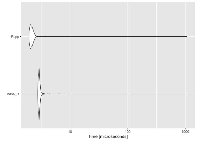
Comparing dist_haversine() with dist_haversine_rcpp(), the compiled version isn’t that much faster. Considering we’re on the scale of microseconds, it really isn’t that much faster.

## time for base R to do many to many with 100 starting points
system.time(dist_mtom(cbg_df$lon[1:100],
                      cbg_df$lat[1:100],
                      col_df$lon,
                      col_df$lat,
                      cbg_df$fips11[1:100],
                      col_df$unitid))

   user  system elapsed 
  2.525   0.012   2.539 

## ...and now Rcpp version
system.time(dist_mtom_rcpp(cbg_df$lon[1:100],
                           cbg_df$lat[1:100],
                           col_df$lon,
                           col_df$lat,
                           cbg_df$fips11[1:100],
                           col_df$unitid))

   user  system elapsed 
  0.045   0.000   0.046 

## compare just 10 many to many
tm_mtom <- microbenchmark(base_R = dist_mtom(cbg_df$lon[1:10],
                                             cbg_df$lat[1:10],
                                             col_df$lon,
                                             col_df$lat,
                                             cbg_df$fips11[1:10],
                                             col_df$unitid),
                          Rcpp = dist_mtom_rcpp(cbg_df$lon[1:10],
                                                cbg_df$lat[1:10],
                                                col_df$lon,
                                                col_df$lat,
                                                cbg_df$fips11[1:10],
                                                col_df$unitid),
                          times = 100L)

## results
tm_mtom

Unit: milliseconds
   expr        min         lq       mean     median         uq        max
 base_R 221.641507 227.737364 236.004614 233.302698 238.464247 308.327211
   Rcpp   3.101263   3.511224   3.764691   3.746062   4.003859   4.796772
 neval
   100
   100

## plot
autoplot(tm_mtom)

Coordinate system already present. Adding new coordinate system, which will replace the existing one.

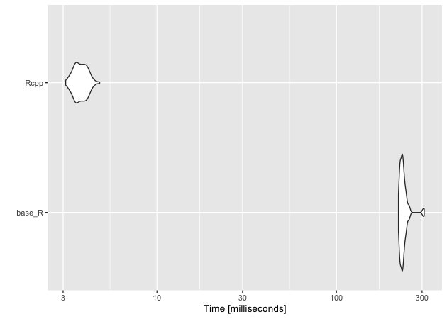
Where we start to see speed improvements in the main function. The compiled version of the many to many function is nearly two orders of magnitude faster!

## time for base R to do many to many with 100 starting points
system.time(dist_min(cbg_df$lon[1:100],
                     cbg_df$lat[1:100],
                     col_df$lon,
                     col_df$lat,
                     cbg_df$fips11[1:100],
                     col_df$unitid))

   user  system elapsed 
  2.478   0.005   2.486 

## ...and now Rcpp version
system.time(dist_min_rcpp(cbg_df$lon[1:100],
                          cbg_df$lat[1:100],
                          col_df$lon,
                          col_df$lat,
                          cbg_df$fips11[1:100],
                          col_df$unitid))

   user  system elapsed 
  0.047   0.001   0.048 

## compare just 10 min
tm_min <- microbenchmark(base_R = dist_min(cbg_df$lon[1:10],
                                           cbg_df$lat[1:10],
                                           col_df$lon,
                                           col_df$lat,
                                           cbg_df$fips11[1:10],
                                           col_df$unitid),
                         Rcpp = dist_min_rcpp(cbg_df$lon[1:10],
                                              cbg_df$lat[1:10],
                                              col_df$lon,
                                              col_df$lat,
                                              cbg_df$fips11[1:10],
                                              col_df$unitid),
                         times = 100)
## results
tm_min

Unit: milliseconds
   expr        min         lq       mean     median         uq        max
 base_R 215.037837 239.062711 247.171698 246.488845 252.828805 317.801239
   Rcpp   3.382741   4.003108   4.223458   4.187064   4.423666   5.330061
 neval
   100
   100

## plot
autoplot(tm_min)

Coordinate system already present. Adding new coordinate system, which will replace the existing one.

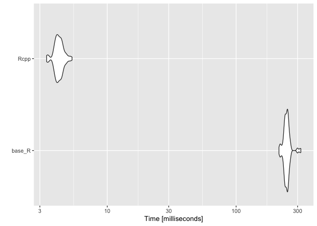
Similarly, the compiled minimum distance function is much faster than the base R function.

In this case as well as the former, we should note that we aren’t comparing fully optimized versions of either function. That said, while it’s possible that the base R functions could be sped up, neither is likely to come close to matching the speed of the compiled Rcpp versions.

Full run for Rcpp version

Throughout, we’ve been running the functions on a reduced starting data set. But how long does it take to find the nearest college to each census block? Let’s find out!

## find minimum
system.time(full_min <- dist_min_rcpp(cbg_df$lon,
                                      cbg_df$lat,
                                      col_df$lon,
                                      col_df$lat,
                                      cbg_df$fips11,
                                      col_df$unitid))

   user  system elapsed 
 75.987   0.144  76.301 

## show
full_min %>% tbl_df()

# A tibble: 217,740 x 3
   fips11       unitid meters
   <chr>        <chr>   <dbl>
010010201001 101471 15786.
010010201002 101471 14229.
010010202001 101471 13949.
010010202002 101471 14870.
010010203001 101471 13363.
010010203002 101471 14390.
010010204001 101471 12705.
010010204002 101471 13271.
010010204003 101471 14102.
010010204004 101471 14757.
# ... with 217,730 more rows

Just a little over two minutes to compute 217,000 by 7,700 distances, finding and storing the minimally distance college along with its distance!

Not-so quick exercise

Below is a function that computes the great circle distance using Vincenty’s formula. It’s more accurate than the haversine version, but can be much more computationally intensive. Try to convert the base R function into an Rcpp function. You’ll need to start a new script and then use sourceCpp() to read it in and test. Once you’ve got, substitute the respective Vincenty formula functions into the dist_min_*() functions and compare times.

A few things to keep in mind:
1. You’ll need to declare your variables and types (lot’s of double); don’t forget that double numbers need a decimal, otherwise C++ thinks they are integers.
2. Don’t forget your semi-colon line endings!
3. abs() in C++ is fabs()
4. Remember: a^2 = a * a

## base R distance function using Vincenty formula
dist_vincenty <- function(xlon,
                          xlat,
                          ylon,
                          ylat) {

    ## return 0 if same point
    if (xlon == ylon && xlat == ylat) { return(0) }

    ## convert degrees to radians
    xlon <- deg_to_rad(xlon)
    xlat <- deg_to_rad(xlat)
    ylon <- deg_to_rad(ylon)
    ylat <- deg_to_rad(ylat)

    ## ---------------------------------------------------
    ## https:##en.wikipedia.org/wiki/Vincenty%27s_formulae
    ## ---------------------------------------------------

    ## some constants
    a <- 6378137
    f <- 1 / 298.257223563
    b <- (1 - f) * a
    U1 <- atan((1 - f) * tan(xlat))
    U2 <- atan((1 - f) * tan(ylat))
    sinU1 <- sin(U1)
    sinU2 <- sin(U2)
    cosU1 <- cos(U1)
    cosU2 <- cos(U2)
    L <- ylon - xlon
    lambda <- L                         # initial value

    ## set up loop
    iters <- 100                        # no more than 100 loops
    tol <- 1.0e-12                      # tolerance level
    again <- TRUE

    while (again) {

        ## sin sigma
        sinLambda <- sin(lambda)
        cosLambda <- cos(lambda)
        p1 <- cosU2 * sinLambda
        p2 <- cosU1 * sinU2 - sinU1 * cosU2 * cosLambda
        sinsig <- sqrt(p1^2 + p2^2)

        ## cos sigma
        cossig <- sinU1 * sinU2 + cosU1 * cosU2 * cosLambda

        ## plain ol' sigma
        sigma <- atan2(sinsig, cossig)

        ## sin alpha
        sina <- cosU1 * cosU2 * sinLambda / sinsig

        ## cos^2 alpha
        cos2a <- 1 - (sina * sina)

        ## cos 2*sig_m
        cos2sigm <- cossig - 2 * sinU1 * sinU2 / cos2a

        ## C
        C <- f / 16 * cos2a * (4 + f * (4 - 3 * cos2a))

        ## store old lambda
        lambdaOld <- lambda

        ## update lambda
        lambda <- L + (1 - C) * f * sina *
            (sigma + C * sinsig * (cos2sigm + C * cossig *
                                   (-1 + 2 * cos2sigm^2)))

        ## subtract from iteration total
        iters <- iters - 1

        ## go again if lambda diff is > tolerance and still have iterations
        again <- (abs(lambda - lambdaOld) > tol && iters > 0)
    }
    ## if iteration count runs out, stop and send message
    if (iters == 0) {
        stop("Failed to converge!", call. = FALSE)
    }
    else {

        ## u^2
        Usq <- cos2a * (a^2 - b^2) / (b^2)

        ## A
        A <- 1 + Usq / 16384 * (4096 + Usq * (-768 + Usq * (320 - 175 * Usq)))

        ## B
        B <- Usq / 1024 * (256 + Usq * (-128 + Usq * (74 - 47 * Usq)))

        ## delta sigma
        dsigma <- B * sinsig *
            (cos2sigm + B / 4 *
             (cossig * (-1 + 2 * cos2sigm^2)
                 - B / 6 * cos2sigm * (-3 + 4 * sinsig^2)
                 * (-3 + 4 * cos2sigm^2)))

        ## return the distance
        return(b * A * (sigma - dsigma))
  }
}

Workshop on R

May 2018

Overview
Schedule
Getting started
Modules
Data

High performance R with Rcpp

Load data

College locations

Census block group locations

Compute great circle distance with Haversine

Quick exercise

Many to many distance matrix

Quick exercise

Nearest end point

Quick exercise

Rcpp

Front matter

Utility functions

Many to many distance matrix

Nearest end point

Source the Rcpp file

Quick comparisons

Single distance

Many to many

Minimum distances

Benchmarks

Full run for Rcpp version

Not-so quick exercise